A slicer is an interactive filter that makes it easy to quickly filter multiple pivot tables and charts. Slicers filter the underlying source data, which dynamically filters everything that references the source data. Slicers are particularly useful for dashboards and summary sheets in large, complex workbooks. Row Zero is an enterprise-grade spreadsheet built for big data. While the process is similar for adding slicers in Excel and Row Zero, Row Zero slicers are much more powerful. Unlike Excel slicers, Row Zero slicers are full-featured, portable filters. You can filter on conditions (e.g. >=5), search values, select all, unselect all, and filter on date groupings like month, week, day, etc. View a live example of slicers in a spreadsheet here or continue reading the slicers tutorial below.
View a live example of slicers
- What is a slicer?
- How to add slicers
- Pivot table slicers
- Pivot chart slicers
- Connected slicers
- Slicers from cell ranges
- How to create dashboard slicers
- Slicers with multiple conditions
- Slicers vs filters
- 5 ways Row Zero slicers are more powerful
What is a slicer?
A slicer is an interactive filter that makes it easy to quickly filter data in pivot tables, pivot charts, or data tables. Slicers filter a pivot table's underlying source data which dynamically filters the pivot table and related charts.  Slicers are particularly useful for dashboards and summary sheets in large, complex workbooks. You can place the slicer next to your charts and pivot tables and it can filter source data on a different sheet, which dynamically filters your pivot charts and tables. They also make it easy for non-technical users to quickly filter data with a few clicks.
View a live example of slicers in a spreadsheet here.
How to add slicers
Row Zero makes it easy to add slicers to pivot tables, pivot charts, data tables, and cell ranges. To add a slicer, simply select your data and go to 'Insert' in the header navigation and select 'Slicer'. 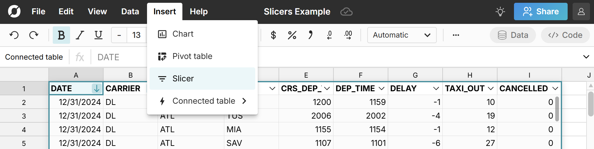
Pivot table slicers
You can add pivot table slicers that filter either the pivot table output or the pivot table source data. It's typically most useful to add a slicer to pivot table source data and then place the slicer next to the pivot table. Here's how:
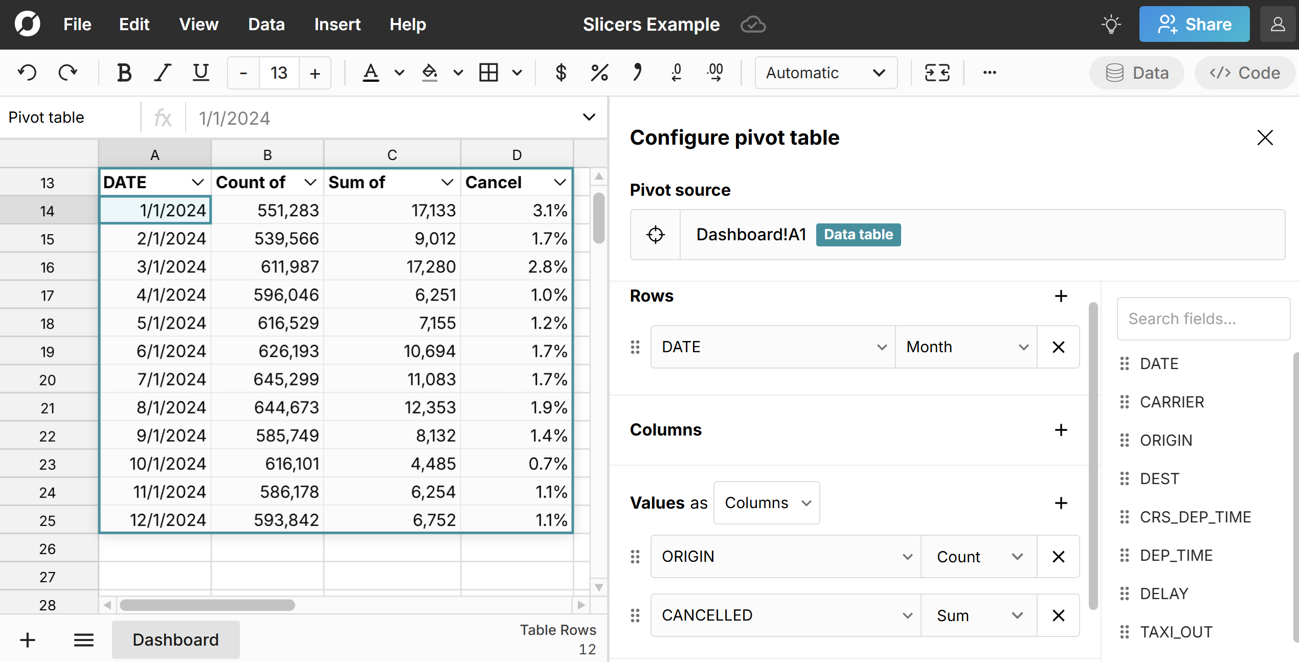
- Create a pivot table from a data table or a cell range with filters applied.
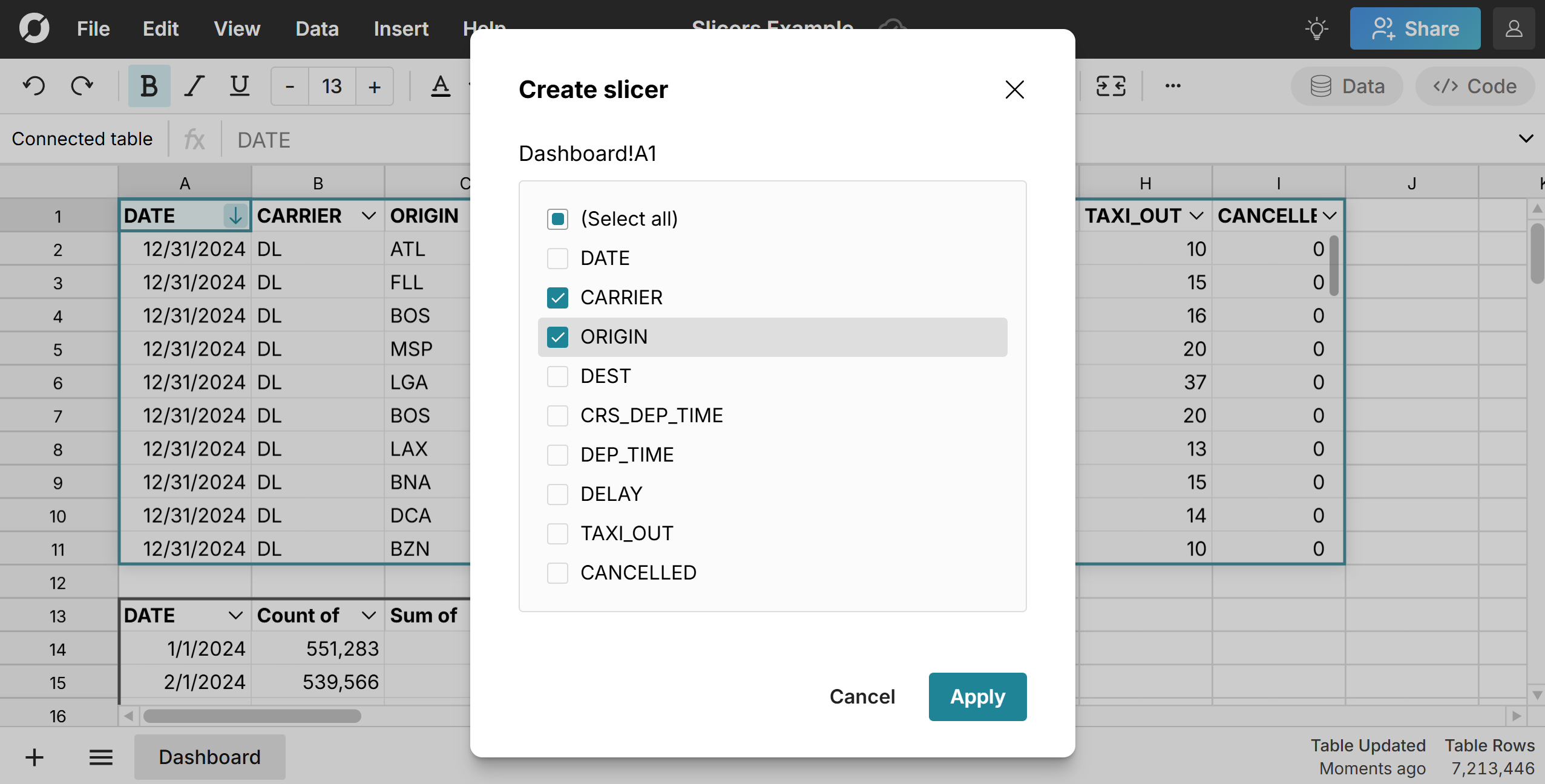
- Navigate back to your source data, click on a cell in the data and go to 'Insert', 'Slicer', and select each column to create a slicer for. Click 'Apply'.
- A slicer is created for each column selected. Click in the dropdown to filter the slicer. You can select from the list of values, search for a value, or filter by condition (e.g. >=5). Click 'Apply' and the source data will filter accordingly and the pivot table dynamically updates with the applied slicer filter.

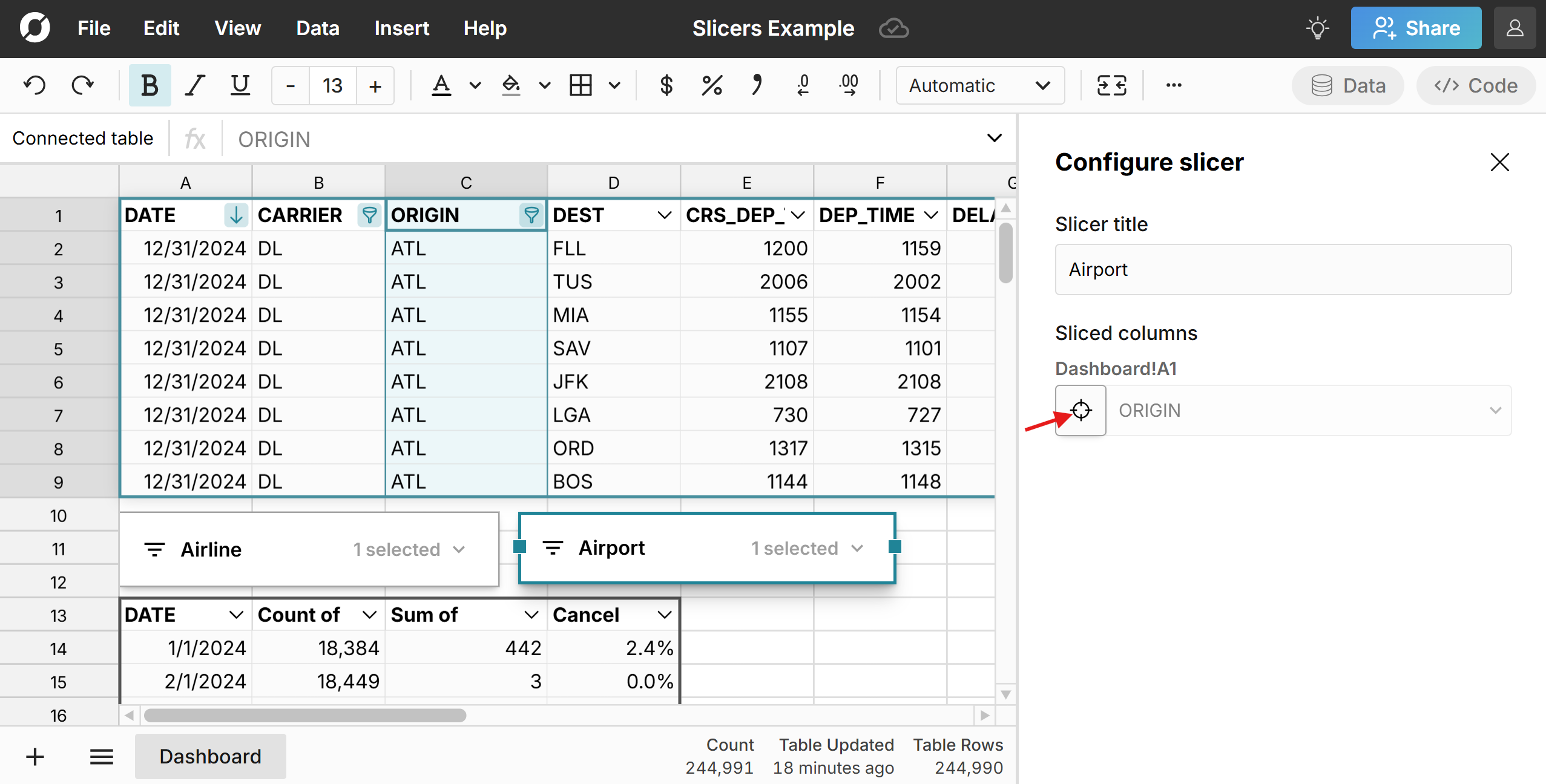
- You can further configure your slicer by double clicking on it. You can rename the slicer and also click on the source icon next to the sliced column to go back to the source range.
 You can also move your slicer around the sheet and right-click to open a context menu where you can delete your slicer, or cut and paste your slicer to another sheet.
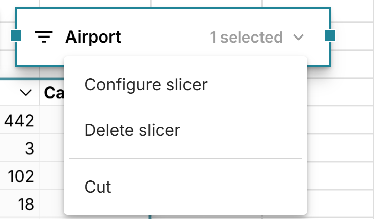
Now that your slicer is created, you can easily apply filters to pivot table source data to dynamically explore your data in a pivot table. You can connect your slicer to multiple pivot tables, charts, formulas, etc. on top of your pivot table data and everything dynamically updates as you change slicer filters.
Adding slicers to pivot table output
In addition to adding slicers to pivot table source data, you can add slicers to the pivot table itself to make it easy to filter pivot table data. Note this is the same as using the built-in pivot table filters, but gives the flexibility of interacting with those filters in a different location (e.g. on a different sheet or next to a pivot chart).
The process is the same as outlined above:
- Click on a cell in your pivot table and go to 'Insert', 'Slicer' in the header navigation to create a pivot table slicer.
- Select the slicer columns and then click in the slicer dropdown to filter by values or conditions.
- Move or cut/paste your slicer to your desired location (e.g. next to a chart or on another sheet).
Pivot chart slicers
Adding slicers to a pivot chart (or any chart) is just as simple. If you've already added a slicer to your pivot table, the slicer will also control any charts you create from the pivot table data. 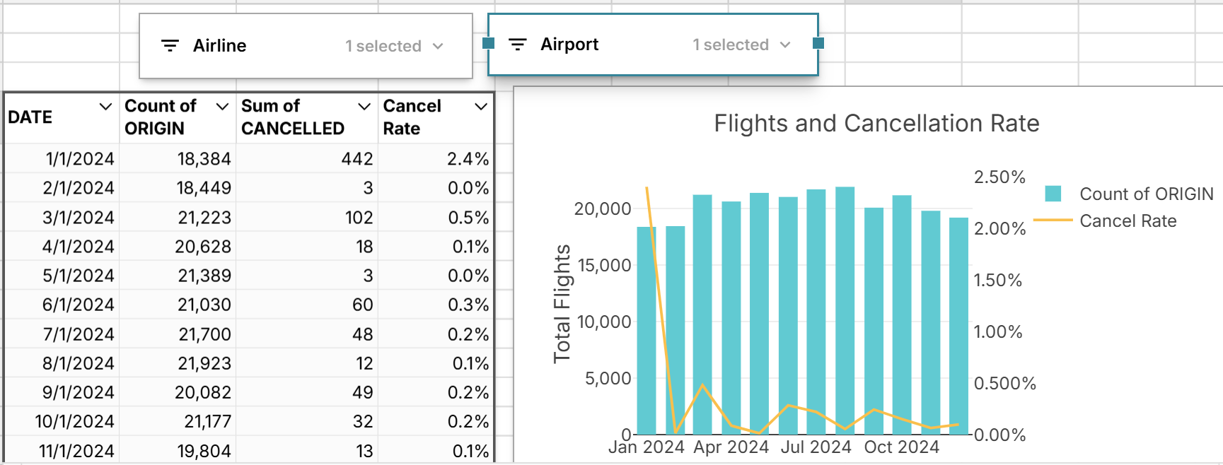 If you haven't yet created a slicer, you can add a chart slicer by adding a slicer to the source data for the chart. If your source data is a cell range, just be sure to first add filters to the range.
Connected slicers that auto-update
Row Zero makes it easy to connect to your data source and build auto-updating spreadsheets. If your source data is a connected table, then any slicers added to the connected table or any pivot table slicers that are built from the connected data will work in sync as your source data updates. You can manually re-run connected tables or schedule auto-refresh to automate updates.
Create slicers from cell ranges
In addition to data tables, you can also create slicers from cell ranges where filters are applied. Simply select your data range, apply filters (if you haven't already), and then go to 'Insert', 'Slicer' to insert a slicer connected to the cell range.
Create dashboard slicers in your spreadsheet
Row Zero makes it easy to create dynamic dashboards connected to your data that auto-update. You can add slicers to your source connected table and it will dynamically filter everything in your dashboard that references it. To create a dashboard slicer, just add the slicer to the connected table and then move it to your desired location on your dashboard by dragging or cut/paste. You can connect slicers to multiple pivot tables and charts and connect slicers across sheets to filter your raw data. 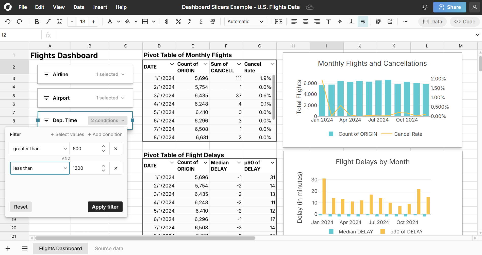
How to connect slicers to multiple pivot tables and charts
It's easy to connect slicers to multiple pivot tables and charts if your pivot tables have the same source data. Simply add a slicer to the source data for your pivot tables and it will control everything that references the source data. As mentioned above, you can use this as a dashboard slicer that controls multiple pivot tables, charts, formulas, etc.
Here's a tutorial of how to create dashboard slicers to filter multiple pivot tables and charts at once:
Slicers across multiple sheets
To move a slicer across sheets, simply right click on the slicer and select 'Cut' and go to your desired location and paste (CTRL+V) the slicer. Filtering the slicer will filter the source data on the other sheet.
Slicers with multiple conditions
Unlike Excel slicers, Row Zero slicers let you filter on conditions like ">=0", before, contains, etc. You can filter slicers using multiple conditions (e.g. ">=0" and "<=10"), so you can filter slicers between dates and numbers. This gives slicers the full functionality of column filters.
Slicers vs filters
In Row Zero, slicers are full-featured, portable filters. Slicers are connected to their underlying filters and actively change the filters applied to the data. 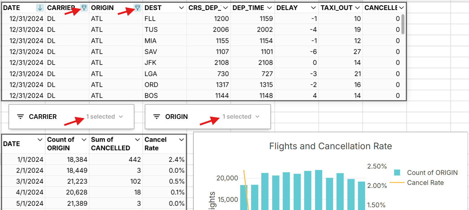
This makes them a lot more powerful than Excel slicers. Row Zero slicers let you easily filter on conditions (e.g. >=5), search values, select all, unselect all, and filter date groupings like month, week, day, etc. Slicers in Excel are not filters and are limited to just selecting values.
Note, because Row Zero slicers are connected to their source filters, if you go to the source data and attempt to adjust the filter, you'll see a message that says "This column's filters are controlled by a slicer". 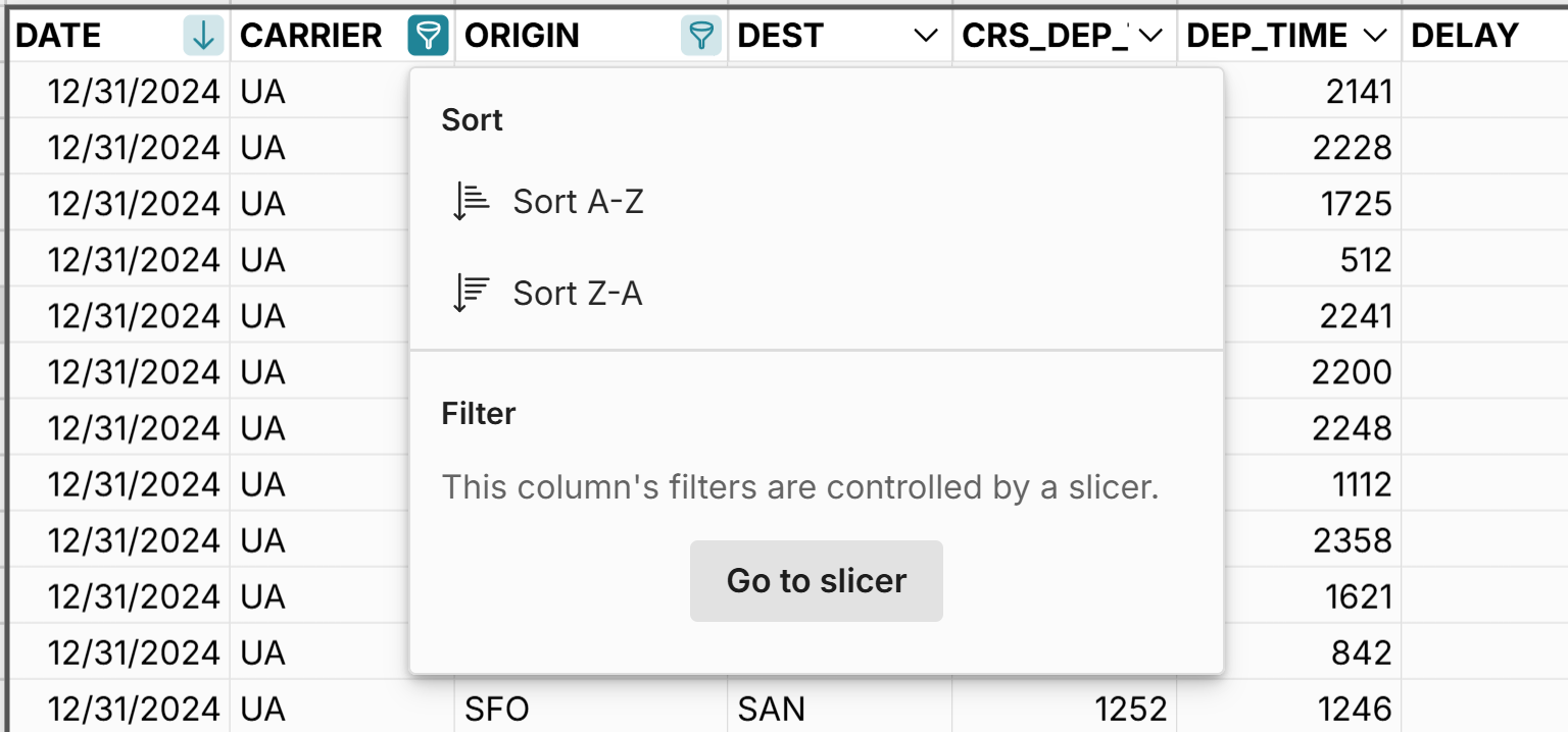 You'll need to delete the slicer to use the source filter again.
5 ways Row Zero slicers are more powerful
Row Zero slicers offer several unique benefits compared to Excel slicers and Google Sheets slicers.
- Big data slicers: Row Zero is 1000x more powerful than legacy spreadsheets and supports billion row spreadsheets on Enterprise plans. Excel slicers are limited to datasets up to the Excel maximum row of 1,048,576 rows. Google Sheets limits are similar.
- Row Zero slicers are full-featured filters: Unlike Excel slicers, Row Zero slicers are full-featured column filters. You can filter slicers by conditions or values, search for values, select all, select none, and clear filters easily. You can also filter slicers by multiple conditions.
- Filter slicers by date groupings like month, week, day, etc. You can also use date slicers between dates by filtering on conditions like before and after.
- Dashboard slicers: You can easily create one slicer for multiple pivot tables and charts, and slicers connect across sheets to filter millions of rows of raw data. The process is a lot simpler than using Report Connections for Excel slicers for multiple pivot tables.
- Connected and auto-updating: Slicers added to connected tables let you filter dynamic data connected to your data source and automate data updates.
Conclusion
Slicers offer a convenient way to filter source data and dynamically filter everything that references that source data including pivot tables, charts, formulas, dashboards, etc. While the process is similar for adding slicers in Excel and Row Zero, Row Zero slicers are much more powerful. Unlike Excel slicers, Row Zero slicers are full-featured, portable filters. You can create dashboard slicers that filter on conditions (e.g. >=5), search values, select all, unselect all, and filter datetime groupings by day, week, month, etc. Row Zero's big data power makes it easy to build dynamic dashboards on massive datasets and slicers make it easy to quickly filter and explore these large datasets. You can view a live example of slicers in a spreadsheet here and try Row Zero for free.