VLOOKUP, short for "vertical lookup," is a spreadsheet function that enables users to search for a value in the leftmost column of a table and retrieve a related value from a column to its right. The VLOOKUP function is a powerful tool in Excel that allows you to search for a specific value in a table and return a corresponding value from another column. Understanding how to use the VLOOKUP function is essential for anyone working with data analysis and spreadsheet management. Read on to learn more about how to use VLOOKUP or skip to specific sections using the table of contents.
- What is VLOOKUP?
- VLOOKUP examples
- Importance of VLOOKUP in data analysis
- Setting up your spreadsheet for VLOOKUP
- Organizing data for VLOOKUP
- Preparing your lookup value
- Step-by-step guide to using VLOOKUP
- Key points to consider with VLOOKUP
- When to use the VLOOKUP function
- VLOOKUP crashes Excel and Google Sheets
- Troubleshooting common VLOOKUP errors
- Conclusion
What is VLOOKUP?
The VLOOKUP function is particularly useful when dealing with large amounts of data and the need to quickly find specific information. Imagine you have a spreadsheet with thousands of rows of data, containing information about customers, products, and sales. Without the VLOOKUP function, finding a specific customer's purchase history or a product's sales performance would be a time-consuming and error-prone task. However, with the VLOOKUP function, you can swiftly search for a customer's name or a product code and retrieve the corresponding information.
The VLOOKUP function is used to retrieve information from a table based on a specified lookup value. There is a new version of VLOOKUP called XLOOKUP that resolves the deficiencies of VLOOKUP. The VLOOKUP function uses the following syntax:
=VLOOKUP(lookup_value, table_array, col_index_num, [range_lookup])
- lookup_value is the value you want to find in the table.
- table_array is the range of cells that contains the data you want to search through.
- col_index_num is the column index of the value you want to retrieve within the table_array.
- [range_lookup] is an optional argument that specifies whether you want an exact match or an approximate match. It's set to TRUE (or omitted) for an approximate match and FALSE for an exact match.
VLOOKUP Examples
Basic VLOOKUP Usage
Suppose you have a table with employee IDs in column A and their corresponding names in column B. To find the name of an employee with ID "E123," use the following formula:
=VLOOKUP("E123", A1:B10, 2, FALSE)
Approximate Match with VLOOKUP
If you have a table with grade ranges and corresponding letter grades, and you want to find the letter grade for a score of 85, use:
=VLOOKUP(85, A1:B5, 2, TRUE)
VLOOKUP for Price Lookup
Imagine you have a product catalog with item codes in column A and their corresponding prices in column C. If you want to find the price of an item with code "P456," you can use:
=VLOOKUP("P456", A1:C10, 3, FALSE)
Importance of VLOOKUP in Data Analysis
Data analysis is a crucial component of decision-making in various fields, including finance, marketing, and operations. It involves examining large amounts of data to uncover patterns, trends, and insights that can inform strategic actions. However, with the ever-increasing volume of data available, it can be challenging to efficiently find and retrieve specific information.
VLOOKUP is an invaluable tool in data analysis as it allows you to efficiently search and retrieve information from large datasets. Whether you are working on financial analysis, sales forecasting, or any other type of data analysis, the VLOOKUP function can significantly streamline your workflow and enhance your analytical capabilities.
One of the key advantages of using the VLOOKUP function is its ability to handle complex data relationships. For example, you may have a dataset with multiple tables, each containing different types of information. By utilizing the VLOOKUP function, you can easily link these tables together based on common identifiers, such as customer IDs or product codes. This enables you to perform comprehensive analyses by combining data from various sources.
Moreover, the VLOOKUP function allows for flexibility in data analysis. You can customize the search criteria to match specific conditions, such as finding the highest or lowest value, identifying duplicates, or filtering data based on certain criteria. This flexibility empowers you to perform advanced data manipulations and gain deeper insights into your dataset.
In conclusion, the VLOOKUP function is a powerful tool in data analysis, enabling users to efficiently search and retrieve information from large datasets. Its ability to handle complex data relationships and provide flexibility in analysis makes it an essential function for any data analyst or professional working with data. By leveraging the VLOOKUP function, you can enhance your analytical capabilities and make more informed decisions based on data-driven insights.
Setting Up Your Spreadsheet for VLOOKUP
Before you can start using the VLOOKUP function, you need to properly organize your data. Here are a few key steps to consider:
When it comes to working with spreadsheets, organization is key. By organizing your data effectively, you can ensure that your VLOOKUP function works smoothly and efficiently. One way to achieve this is by arranging your information in a table format. This means using columns to represent different variables or categories. By doing so, you create a structured and logical layout for your data.
Now, let's talk about the all-important "lookup column." This is the leftmost column in your table, and it contains unique values that you will use to search for specific information. These unique values serve as the foundation for your VLOOKUP function. It's crucial to have these values properly defined and organized so that you can easily find the information you need.
Organizing Data for VLOOKUP
To effectively utilize the VLOOKUP function, it is essential to have your data well-organized. Arrange your information in a table format, with each column representing a different variable or category. Ensure that the leftmost column, also known as the "lookup column," contains unique values that you will use to search for specific information.
By organizing your data in this way, you create a structured and logical layout for your spreadsheet. This not only makes it easier to use the VLOOKUP function but also enhances the overall readability and usability of your spreadsheet.
Additionally, consider labeling your columns with clear and descriptive headers. This will make it easier for you and others to understand the purpose of each column and the type of data it contains. Clear labeling is especially important when working with large datasets or collaborating with others.
Preparing Your Lookup Value
Before entering the VLOOKUP formula, you should establish the value you want to search for in the lookup column. This value could be a specific number, text, or even a cell reference within your spreadsheet.
When selecting your lookup value, it's important to choose something that is unique and specific. This will ensure that the VLOOKUP function returns accurate and relevant results. Take the time to carefully consider the value you want to search for and ensure that it aligns with the purpose of your spreadsheet.
Remember, the success of the VLOOKUP function relies heavily on the quality of your data and the accuracy of your lookup value. By taking the time to properly prepare and organize your spreadsheet, you set yourself up for success when using the VLOOKUP function.
Step-by-Step Guide to Using VLOOKUP
Now that you have your data organized and your lookup value ready, let's take a closer look at the process of using the VLOOKUP function:
The VLOOKUP function is a powerful tool in Excel that allows you to search for a specific value in a table and retrieve information from that table based on the search criteria. It can be extremely useful when you have large amounts of data and need to quickly find specific information.
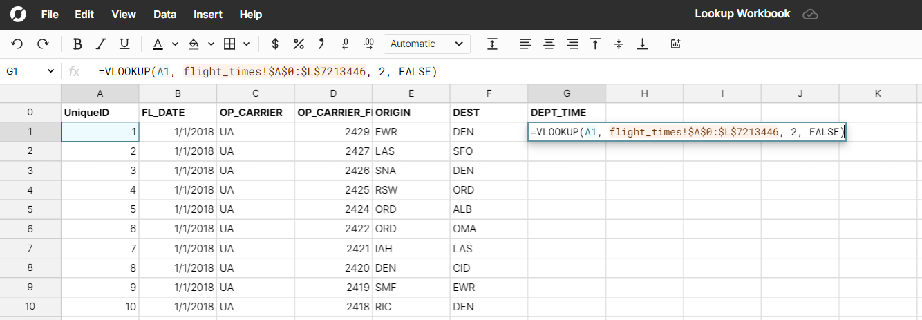
Entering the VLOOKUP Formula
To begin, select the cell where you want the lookup result to appear. Next, enter the VLOOKUP formula using the following syntax: =VLOOKUP(lookup_value, table_array, col_index_num, [range_lookup])
The lookup_value is the value you want to search for in the table. This can be a specific value or a cell reference to a value in another part of your worksheet. The table_array refers to the range of cells that contain your data. Specify the range by selecting the appropriate columns and rows that encompass your data.
The col_index_num is a parameter that determines which column to retrieve the value from in the table array. Count the columns from the leftmost column of the table array to identify the correct index number. This number will determine which column's value will be returned as the result of the VLOOKUP function.
Lastly, the range_lookup parameter determines whether you want an exact match or an approximate match in the lookup process. If you set it to "TRUE" or omit it altogether, Excel will assume an approximate match. This means that if an exact match is not found, Excel will return the closest match that is less than the lookup value. For an exact match, use "FALSE".
Defining the Lookup Range
In the VLOOKUP formula, the table array refers to the range of cells that contain your data. Specify the range by selecting the appropriate columns and rows that encompass your data.
It is important to ensure that the table array is properly defined to include all the relevant data. If the table array is not correctly defined, the VLOOKUP function may return inaccurate results or produce an error.
Specifying the Column Index Number
The col_index_num is a parameter that determines which column to retrieve the value from in the table array. Count the columns from the leftmost column of the table array to identify the correct index number.
It is crucial to accurately specify the column index number to ensure that the VLOOKUP function retrieves the desired information. If an incorrect index number is provided, the function may return incorrect data or produce an error.
Choosing the Range Lookup Value
The range_lookup parameter determines whether you want an exact match or an approximate match in the lookup process. If you set it to "TRUE" or omit it altogether, Excel will assume an approximate match. This means that if an exact match is not found, Excel will return the closest match that is less than the lookup value.
On the other hand, if you set the range_lookup parameter to "FALSE", the VLOOKUP function will only return an exact match. If no exact match is found, Excel will return an error value (#N/A).
When deciding whether to use an approximate or exact match, consider the nature of your data and the specific requirements of your analysis. An approximate match can be useful when dealing with numerical data or when you want to find the closest match. However, if you require precise results and only want an exact match, be sure to set the range_lookup parameter to "FALSE".
Key Points to Consider with VLOOKUP
- The VLOOKUP function is useful for quickly retrieving information from a dataset without manual searching.
- It is commonly used for tasks like data validation, creating summary reports, and consolidating/joining information from different sources.
- VLOOKUP is limited to vertical lookups and requires the lookup value to be in the first column of the table_array.
- In cases where the data isn't sorted or you need more flexible lookup options, consider using the XLOOKUP() function.
When to Use the VLOOKUP Function
- When you need to find specific data points in a large dataset using a single criterion.
- For tasks such as creating reports, summarizing data, and validating input values.
- In situations where you have a well-structured dataset with lookup values in the first column.
- When you want to combine fields from two datasets
VLOOKUP Crashes Excel and Google Sheets
VLOOKUP is a memory intensive function. When running a VLOOKUP over large data sets of 100k rows in Excel or 10k rows Google sheets, the spreadsheet can freeze or crash. The cause of poor performance with VLOOKUP is due to the function's design. VLOOKUP searches every row in the data set looking for a match. As the data set grows, there are more pieces of data to look through, thus increasing the memory requirement on the computer. If VLOOKUP is crashing your Excel file or Google Sheets workbook, try using Row Zero, a powerful spreadsheet designed for big data sets.
Troubleshooting Common VLOOKUP Errors
While the VLOOKUP function is incredibly useful, it is not without its quirks. Here are a few common errors you may encounter:
Dealing with #N/A Errors
An #N/A error indicates that the VLOOKUP function could not find an exact match for the lookup value. Double-check your data and ensure that the value you are searching for exists in the lookup column.
Correcting #REF! Errors
If you encounter a #REF! error, it means that your table array reference is incorrect. Verify that the range you specified in the VLOOKUP formula encompasses the entire table.
Fixing #VALUE! Errors
#VALUE! errors occur when one of the input values within the VLOOKUP formula is not recognized as a valid data type. Ensure that all your cell references and input values are correctly formatted.
Conclusion
The VLOOKUP function is a fundamental tool for data retrieval and analysis in spreadsheets. Its ability to quickly fetch information based on a lookup value makes it indispensable for various business and analytical tasks. While it's primarily used for vertical lookups, VLOOKUP remains a key function for efficiently handling structured data. Experiment with the VLOOKUP function in your Row Zero workbook to explore its capabilities further.