Conditional formatting is a powerful feature that lets you highlight and format cells based on conditions. Row Zero supports conditional formatting with formulas and functions, which offers a wide range of options for formatting your data. In this guide, we'll show several examples of how to apply conditional formatting based on another cell's values using formulas. You can also view live examples here in Row Zero, a powerful spreadsheet for big data.
View conditional formatting formula examples
How to use conditional formatting with formulas
Conditional formatting formulas let you apply conditional formatting based on another cell's values. You can also use functions in conditional format formulas to greatly expand your formatting options. There generally two ways to apply conditional format formulas:
- Select a Condition (e.g. Greater than) and set the value to a formula
- Select "Custom formula" as the Condition and then write a formula
There are a few important considerations with conditional formatting formulas:
- Format formulas evaluate starting in the top-left cell of the format range.
- If you do not use absolute references (e.g. $A$1), the conditional format formulas "drag" down and to the right across the format range.
- Each time the formula evaluates as TRUE, the conditional formatting is applied.
Below, we walk through several examples of how conditional formatting formulas work.
Formatting formula examples
You can view the examples below in a live spreadsheet here.
Conditional format formulas with relative references
In the example below, we want to highlight cells in the Feb column that are greater than the Jan column, so we select our Feb column (C3:C7), click the 3-dots in the sub-menu, click the conditional formatting icon, and select 'New rule'.
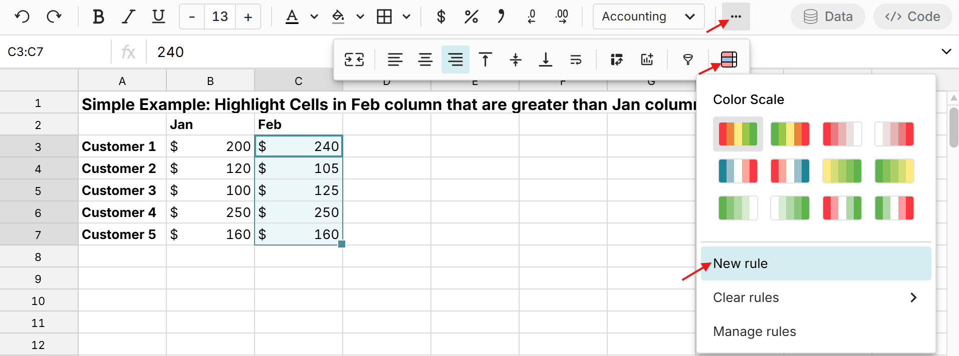 Select "Greater Than" for the condition, enter the formula "=B3" (the first cell to evaluate against), and then select your desired formatting.
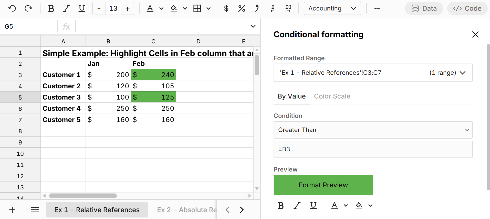
The conditional formatting starts at the top-left cell of the format range (C3:C7), which is C3, and evaluates if 'Greater than' the formula '=B3'. In this case, 240 is greater than 200, so the formatting is applied. The format formula drags down automatically, so for example, cell C5 evaluates as greater than B5 and the conditional formatting is applied.
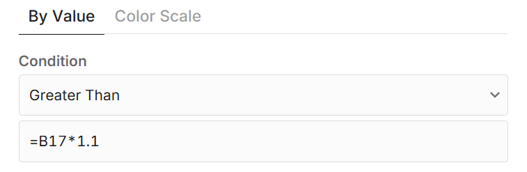
Conditional format formula that drags across range
The example above only looked at one column. In the example below we show how conditional format formulas drag down and to the right across the range. 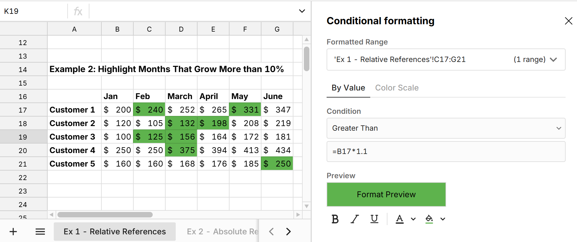
The conditional formatting starts at the top-left cell of the format range (C17:G21), which is C17, and evaluates if 'Greater than' the formula "=B17 times 1.1'. If TRUE, the formatting is applied. The formula drags down and to the right across the range. So cell G21 evaluates as greater than '=F21 times 1.1' and the conditional formatting is applied.
Conditional format formulas with absolute references
If you don't want your conditional format formulas to drag across the range, you need to use "$" to set absolute references. In the example below, we set the condition to "Greater Than" the absolute reference of "=$B$5". This evaluates every cell in the format range against cell B5 and applies formatting when greater. 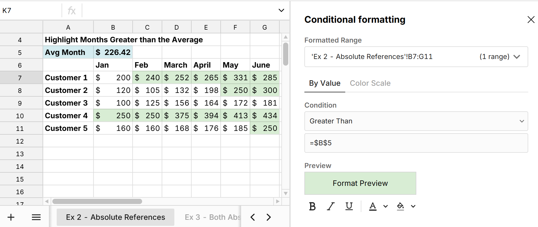 Using absolute references lets you apply conditional formatting based on another cell, without the reference moving with the range as shown above.
Conditional formatting based on another row or column
We can use a combination of absolute and relative references to apply conditional formatting based on another column or row. 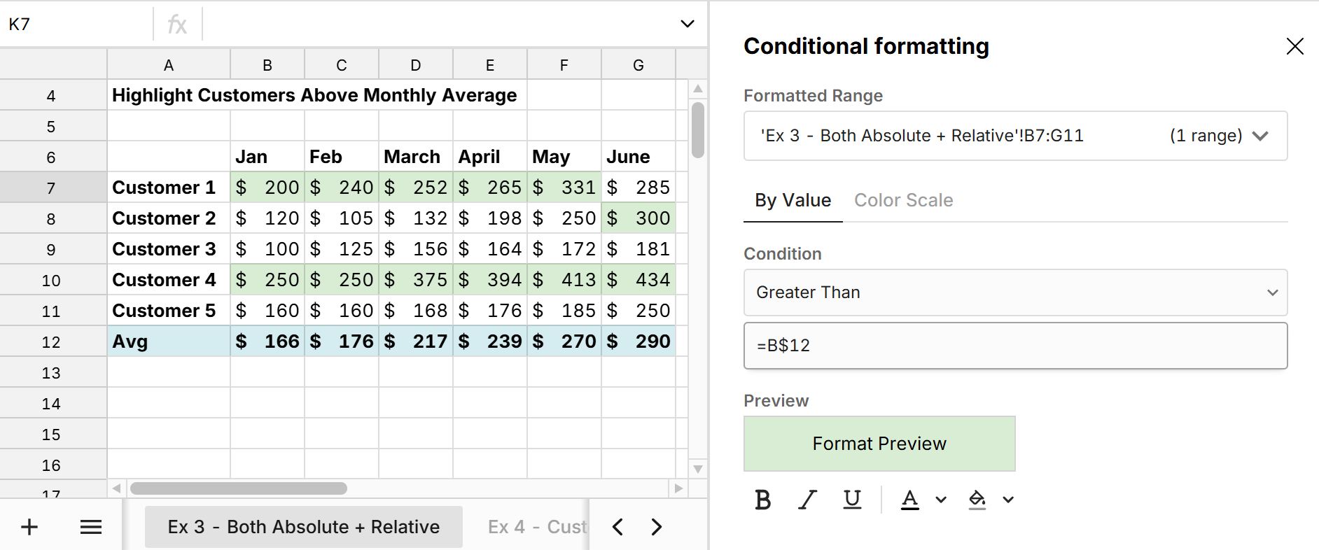 In this example, the formatting starts at the top left of the format range (B7:G11) and evaluates if greater than B$12. Since the formula uses a $ sign in front of 12 but not in front of B, row 12 is an absolute reference and column B is a relative reference. As a result, the formula drags to the right across columns in row 12. For example, cell G10 evaluates the format formula as 'Greater than' '=G$12', which is TRUE and the formatting is applied.
To apply conditional formatting based on a column, you need to make your column reference absolute.
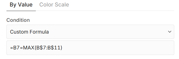
Conditional formatting with custom formulas
You can create custom conditional formatting rules by setting the Condition to "Custom formula". In the example below, we format the max value in each column. 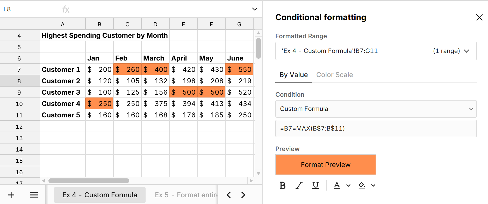 The conditional formatting starts at the top-left cell of the format range (B7:G11) and applies the custom formula '=B7=MAX(B$7:B$11)', which evaluates whether B7 is the MAX of the values in B7 to B11. This formula drags down and to the right, evaluating each cell in the format range, but since a '$' is before the 7 and 11, the rows are absolute references, so the formula always looks for the MAX for the given column between rows 7 and 11.
Conditional format entire row
Custom formulas make it easy to apply conditional formatting to an entire row. Ensure the entire row is in the formatted range and make the column reference absolute in the formula using '$'. 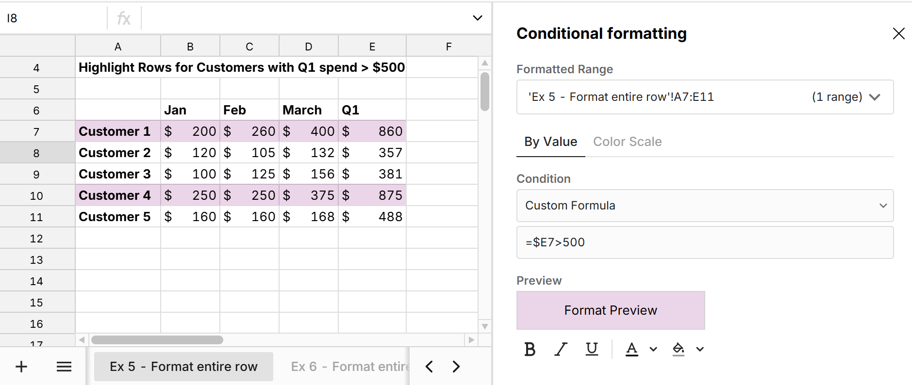 In this example, the conditional formatting starts at the top-left cell of the format range (A7:E11) in cell A7 and evaluates the format formula '=$E7 > 500'. This evaluates to TRUE so cell A7 is formatted. Since column 'E' is an absolute reference and row 7 is a relative reference, the formula format will always look at column E but will drag down to each row. So everything in A7:E7 evaluates the formula '=$E7 > 500' which is TRUE so the entire row is formatted. For the next row, everything in A8:E8 evaluates the formula '=$E8>500' which is FALSE, so every cell in this row is not formatted.
Conditional format entire column
You can similarly apply conditional formatting to an entire column by making the row reference absolute in your formatting formula. 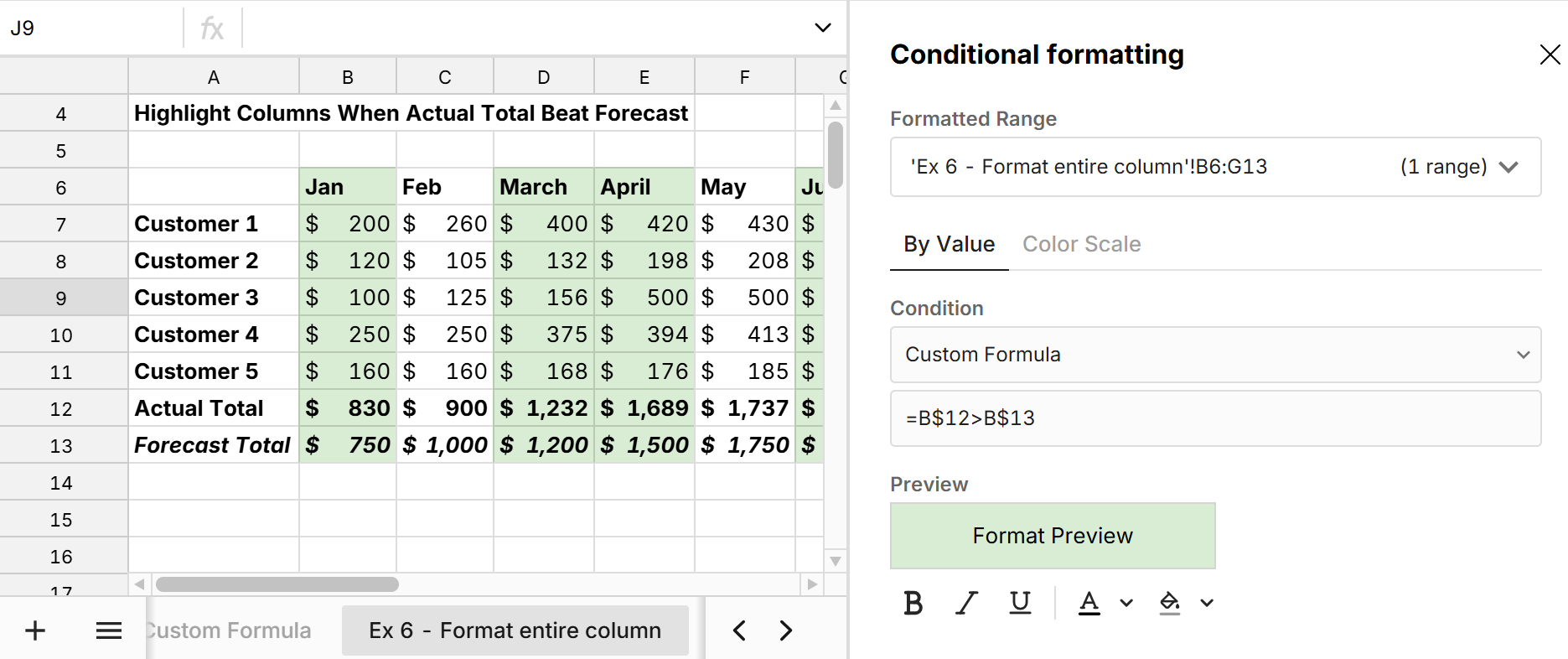 The conditional formatting starts at the top-left cell of the format range (B6:G13) in cell B6 and evaluates the format formula 'B$12>B$13'. This evaluates to TRUE so cell B6 is formatted. Since rows $12 and $13 are absolute references and column B is a relative reference, the formula format will always look at rows 12 and 13, but will drag across each column. So everything in B6:B13 evaluates the formula '=B$12>B$13' which is TRUE so the entire column is formatted. For the next column, everything in C6:C13 evaluates the formula '=C$12>C$13' which is FALSE, so every cell in this column is not formatted.
Conditional formatting pivot tables and connected tables
Conditional formatting works a bit differently in data tables (pivot tables, connected tables, etc.). You can only apply conditional formatting to one column at a time and formatting is always applied to the full column. You have the option to apply formatting to the entire row. You can reference other columns in the table in your formatting formula with the syntax {column name}. 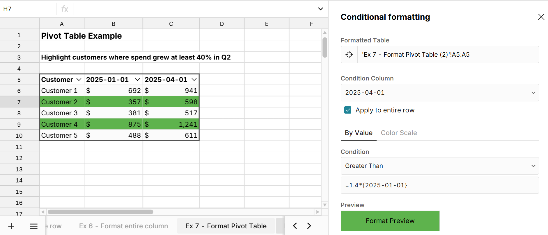 In this example we select 'Greater than" for the Condition and set the formula to =1.4*{2025-01-01} to highlight where Q2 (2025-04-01) is at least 40% greater than Q1 (2025-01-01).
Note at any time, you can use the ARRAY formula to spill your table into cells and get greater flexibility with conditional formatting.
Conclusion
Conditional formatting using formulas gives you endless options to format your data. You can easily apply conditional formatting based on another cell, column, or row and use functions in conditional formatting formulas. You can also use the "Custom formula" condition to write custom conditional formatting rules. By default, conditional format formulas drag across the format range, but you can use "$" to set absolute references, so formatting is based on a specific cell or range.
If you're working with large datasets, it can be a challenge to apply complex conditional formatting formulas in Excel or Google Sheets due to their data limits. In particular, complex conditional formatting can slow down Excel and Sheets. Row Zero is an enterprise-grade spreadsheet built for big data that makes it easy to apply complex conditional formatting rules using formulas and functions across large datasets.